Picture this scenario: you are building a forecasting tool that leverages time series data and you are deciding on your features. Inevitably you get to the question: how do I handle my cyclic variables such as day of year, day of week, and time of day? These features, whilst not exceptionally explainable, tend to provide a lot of predictive power and should variably go into your model if you don’t have access to the true feature. So what do you do with them? Well we have several options in our toolkit. The first is to take delve into the forecasting realm and use models such as ARIMA, or RNNs. These are great models and are commonly used. However, I’d argue that the most common approach is to just hot encode the cyclic variables and run them through a machine learning pipeline. I think we can do better. We can borrow some approaches from forecasting analysis and use Fourier transforms. This dramatically reduces the dimensionality of the data and provides similar results in less time.
What are Fourier transforms?
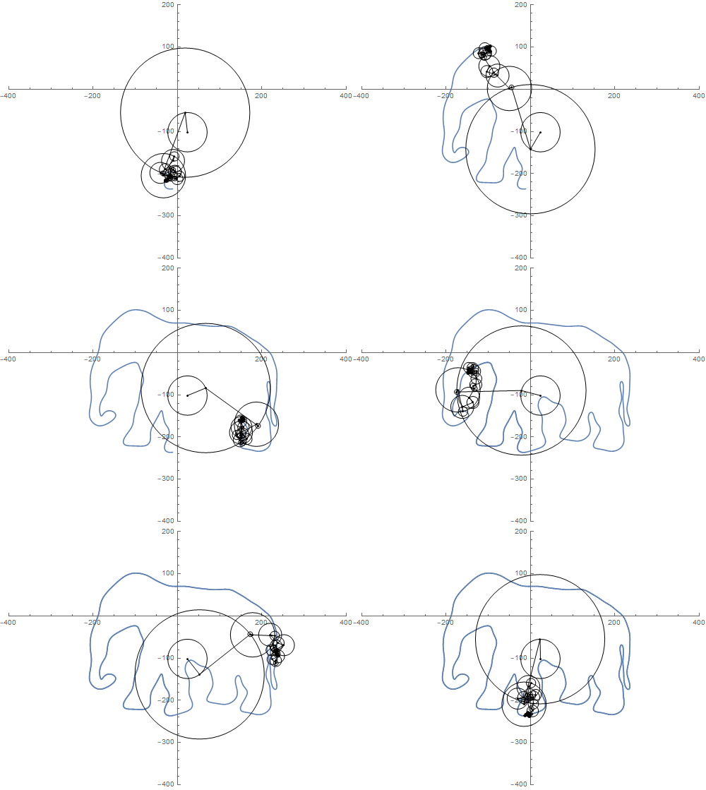
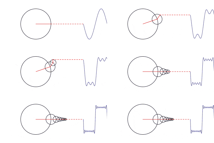
“The Fourier transform (FT) decomposes a function of time (a signal) into its constituent frequencies”. The gist is that functions of time can be expressed as additively combined trigonometric functions. We can then easily decompose them to use in regression. There are some amazing examples of this used in complex ways:

We can leverage this theorem by taking our cyclical variables and perform vector decomposition to create two orthogonal features. More about how to do this shortly.
Let’s go through the process of decomposing the cyclical features into Fourier terms and also the hot encoded version as our benchmark.
Set up environment
For this benchmark, I am going to use some data from the tsibble package. The tsibble package provides a couple of relatively clean time series data-sets that are easy to work with. We will use the pedestrian dataset. The dataset contains the count of pedestrians over a two year period in Melbourne.
library(dplyr)
library(purrr)
library(plotly)
library(DT)
library(forcats)
library(lubridate)
library(rsample)
library(recipes)
library(modelr)
library(broom)
library(yardstick)
library(testthat)


my_dat <-
  tsibble::pedestrian %>%
  as_tibble() %>%
  filter(Sensor == "Birrarung Marr") %>%# shirnking the data for speed
  select(Date_Time, Time, Count) %>%  # extract three common cyclic variables
  mutate(day_of_week = wday(Date_Time),
         month_of_year = month(Date_Time),
         Time        = Time)

my_dat_split <- my_dat %>%
  initial_time_split() # split into train-test sets for future benchmarking/validation

my_dat %>%
  plot_ly(x = ~Date_Time, y = ~Count, type = 'scatter', mode = 'lines')
Based on a quick exploration of the time series, we see cyclic variables that appear based on time of day, day of week and time of year. We also have some missing periods, but we will ignore them for now.
Feature Engineering using Hot Encoding
If you are coming from python you may notice that I am not using a hot encoder. This is because R doesn’t use that terminology and most modeling functions do it implicitly when you pass a factor variable. For explicitness, I went ahead and used moderlr::model_matrix to showcase what the feature matrix looks like prior to modelling. I have subset the matrix for viewing, but you can see that is a very sparse matrix.
In this example, we have 41 features. The pedestrian data does not have readings every day of the year and model_matrix or factoring removes one level per feature so we don’t fall prey to the dummy variable trap. Since R creates the dummies implicitly, we can show what the model data actually looks like with model_matrix, However, we will let R do this for us when running models.
Feature Engineering using Vector Decomposition
Now let’s move on to the feature engineering using the Fourier transforms we discussed earlier. To do this we need a couple inputs:
- The magnitude of the vector
- The length of the cycle
The magnitude of the vector is easy in this case. Since our cyclic term is time, it has no variance in the magnitude and we can just use 1. magnitude does matter in other cyclic terms like wind speed. The length of the cycles are pretty straight forward and are shown in the code chunk below. Again, I have subset the model matrix for viewing.
| Count | hod_sin | hod_cos | dow_sin | dow_cos | moy_sin | moy_cos |
|---|---|---|---|---|---|---|
| 1630 | 0.0000000 | 1.0000000 | -0.9749279 | -0.2225209 | 0.5 | 0.8660254 |
| 826 | 0.2588190 | 0.9659258 | -0.9749279 | -0.2225209 | 0.5 | 0.8660254 |
| 567 | 0.5000000 | 0.8660254 | -0.9749279 | -0.2225209 | 0.5 | 0.8660254 |
| 264 | 0.7071068 | 0.7071068 | -0.9749279 | -0.2225209 | 0.5 | 0.8660254 |
| 139 | 0.8660254 | 0.5000000 | -0.9749279 | -0.2225209 | 0.5 | 0.8660254 |
| 77 | 0.9659258 | 0.2588190 | -0.9749279 | -0.2225209 | 0.5 | 0.8660254 |
| 44 | 1.0000000 | 0.0000000 | -0.9749279 | -0.2225209 | 0.5 | 0.8660254 |
| 56 | 0.9659258 | -0.2588190 | -0.9749279 | -0.2225209 | 0.5 | 0.8660254 |
| 113 | 0.8660254 | -0.5000000 | -0.9749279 | -0.2225209 | 0.5 | 0.8660254 |
| 166 | 0.7071068 | -0.7071068 | -0.9749279 | -0.2225209 | 0.5 | 0.8660254 |
In this case we have 7 features which is considerably less than the model matrix using the hot encoder. We are additively stacking harmonic terms as a way to model the whole. Rather than giving our model lots of different one off cases to handle separately.

Model Performance and Comparison
To compare these two model specs, we will use a simple linear regression and will look at several metrics:
- R squared
- RMSE and MAE on the test set
- Fitting speed
Hot Encoding Method
lm_hot_encode <- lm(Count ~ ., data = in_dat_hot_encode)Out of Sample Test
We are seeing a pretty poor model fit even with all of the terms we included. This is expected with this being a toy problem. There is plenty we could do to improve this model such as flag holidays or use a different type of model entirely but this provides a good benchmark.
test_dat_hot_encode <- my_dat_split %>%
  testing() %>%
  feature_eng_he()

pred_hot_encode <- test_dat_hot_encode %>%
  add_predictions(lm_hot_encode) %>%
  metrics(truth = Count, estimate = pred)

pred_hot_encode %>%
knitr::kable()| .metric | .estimator | .estimate |
|---|---|---|
| rmse | standard | 587.6252339 |
| rsq | standard | 0.2342033 |
| mae | standard | 329.0664334 |
Vector Decomposition Method
Now let’s perform the same test using Fourier terms.
lm_decomp <- lm(Count ~ ., data = in_dat_decomp)Out of Sample Test
So with a linear regression, we see extremely similar if not a little better results using Fourier terms with considerably fewer terms. As expected, this provides an elegant solution to seasonality.
test_dat_decomp <- my_dat_split %>%
  testing() %>%
  feature_eng_decomp()

pred_decomp <- test_dat_decomp %>%
  add_predictions(lm_decomp) %>%
  metrics(truth = Count, estimate = pred)

pred_decomp %>%
knitr::kable()| .metric | .estimator | .estimate |
|---|---|---|
| rmse | standard | 576.3562874 |
| rsq | standard | 0.2276841 |
| mae | standard | 307.5120931 |
Speed Benchmark
To benchmark our model fitting speed and memory, we will use the bench package and run each model 50 times.
We can see from the beeswarm plot that the decomposition method is 0.008 whereas hot encoding is 0.051. The memory allocated in decomposition is 4.02290410^{6} and hot encoding uses 9.92430410^{6}. In general, decomposing cyclic variables is a huge speed up and uses a lot less memory!
Predictions
As a sanity check, we can view the time series and compare the decomposition method, hot encoding, and the actual pedestrian counts per hour. Neither model is fully capturing the large spikes and we have the issue of showing negative counts. This is becuase we are modelling count data with a linear regression which isn’t really the right tool. We could potentially alleviate these problems by using a Poisson model or a decision tree based approach, but that is for another time. The hot encoding method might be performing slightly better during high counts but it is effectively a wash.
In general, using Fourier terms gives similar results with a large increase in computational efficiency. This is especially useful when you have values with long cycles such as weeks per year. When your cyclic variables are short, it is less effective and I would argue that hot encoding is more explainable. I hope you learned something and if you have any questions, please contact me at eric.stern1@gmail.com.